1 Introduction This article discusses the principles, implementation methods and simulation results of adaptive feedforward linearization technology.
To provide uninterrupted supply of power in home, the V-Guard Digital UPS requires the best battery. The VT180 batteries, manufactured by V-Guard, are a perfect fit with the Digital UPS. These batteries also work effectively with other UPS. With a capacity of 180Ah C20 at 27degree C, these batteries offer backup that varies from three hours to fifty four hours depending on the connected load. With a length of 503mm, width of 188mm and height of 417mm, these batteries have a dry weight of 40Kg, filled weight of 64Kg and their gross weight is 66Kg. These batteries can hold 18.5litres of acid, more or less. These batteries come packed in multi coloured cartons. While there is the standard warranty of 36months, prorated warranty of 18months is also available. These are low maintenance batteries designed to provide up to 40% extra backup.
120Ah 12V Solar Battery,120Ah Solar Battery,Solar Battery Yangzhou Bright Solar Solutions Co., Ltd. , https://www.solarlights.pl
Commonly used linearization techniques include feedback method, predistortion method, feedforward method, Cartesian loop, and linearization of nonlinear components (LINC). The predistortion method is the most commonly used, and its working function predistorter has two significant characteristics: linear correction is before the power amplifier, and its insertion loss is small; the bandwidth limit of the correction algorithm is small. The high complexity of digital predistortion technology can provide better IMD compression, but because of the DSP operation speed, its bandwidth is small. Cartesian feedback complexity is low, it can provide reasonable IMD compression, but there are stability problems and the bandwidth is limited to a few hundred kHz. The LINC method turns the input signal into 2 constant envelope signals, which are amplified by two Class C amplifiers and then synthesized, but are sensitive to component drift. Feedforward technology is another type of linearization technology. He provides linearization accuracy of closed-loop systems, stability and bandwidth of open-loop systems. At present, only feed-forward technology can meet the performance indexes of modern multi-carrier communication base station power amplifiers.
The feedforward technology originates from "feedback". It should be said that he is an old technology. In addition to the calibration (feedback) added to the output, the concept is "feedback", but it is a different implementation method. Feedforward overcomes the effects of delay. He provides the advantages of feedback, but does not have the disadvantages of instability and limited bandwidth.
2 Adaptive feedforward method linearization principle
Figure 1 shows the basic feed-forward loop block diagram. The undistorted sampled signal is delayed and compared with the signal amplified by the main amplifier after proper attenuation coupling in a 0 ° to 180 ° synthesizer. If the main amplifier has no gain and phase distortion, the synthesizer produces zero output. If the main amplifier has any gain and phase distortion, compression or AM-PM effects, there will be a small RF error signal at the output of the synthesizer. The input to the error amplifier is amplified to the level of the output sample signal. The main signal is delayed and compensated for errors After the delay of the amplifier is combined with the output of the error amplifier and output after calibration. It must be emphasized that the calibration of phase and amplitude—addition or subtraction—are all performed under RF, not video or baseband. That is, the calibration is performed within the final bandwidth. The final bandwidth is determined by the tracking characteristics of the phase and amplitude of the various components of the system. 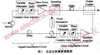
The working principle of this system is well understood, and quantitative analysis requires in-depth discussion, including the analysis of the power capacity of the main power amplifier and the error power amplifier, the nonlinear contribution of the error amplifier; the impact of imperfect gain and phase tracking characteristics. The simplest way is to first analyze the static characteristics of the loop when the main amplifier has gain compression and AM-PM conversion distortion while continuous wave scanning. The so-called "static" is defined as the distortion characteristics of the system under variable envelope excitation.
3 Adaptive feedforward control method
In recent years, there have been some patents for adaptive feedforward systems. These adaptive feedforward technologies are mainly divided into two categories: adaptive methods with or without control signals, that is, adaptive technologies based on power minimization and gradient signal based Adaptive technology. The former control scheme is: in the signal cancellation circuit part, by adjusting the complex vector modulator to minimize the power of the error signal in the frequency band where the reference signal is located, in the error cancellation circuit part, the frequency band containing only the distortion part is selected. Once the optimal parameters are obtained, the pre-prepared disturbances need to be added to update the coefficients. These disturbances reduce IMD compression. The adaptive method using gradient signals is to continuously calculate the gradient of the three-dimensional power surface. The power surface in the signal cancellation circuit is the power of the error signal. When the reference signal is completely compressed and only distortion is left, the power is the smallest. The power surface in the error cancellation circuit is the output power of the linearizer. When the distortion is completely compressed in the output signal of the power amplifier, the power reaches the minimum. The gradient is calculated continuously, so no disturbances prepared in advance are required. Commonly used adaptive controllers include complex gain controllers and minimum power controllers.
There are two main types of typical complex gain regulators: polar and rectangular coordinates. The former consists of attenuator and phase shifter. The latter consists of a power divider, a synthesizer, a phase shifter and a mixer, where the mixer can be replaced with a two-phase voltage controlled attenuation (VCA). The two branches of vector modulation are phase integration, and VCA can work in two phases, which ensures that the vector modulation can obtain a phase shift within [0,360]. The attenuator is set to a normalized value, where the voltage gradient is the largest, so as to ensure fast adaptation, but it must be ensured that no additional nonlinearity is introduced.
The minimum power controller, this adaptive controller is a typical representative of the "minimum power" principle applied to the feedforward linearization technology. Figure 2 is a block diagram of the minimum power controller. The power of port "P" is minimized by adjusting the control voltages "I" and "Q". Port P is a sample of the error signal in the signal cancellation circuit. The disadvantage of this method is that when it reaches the minimum quickly, it converges slowly and is sensitive to measurement noise. The power measurement inevitably has noise. In order to reduce the measurement changes, it needs to stay enough time at each step. The principle of power minimization is also applied to the error cancellation circuit. However, the output signal of port P has both amplified signals and residual distortion. Because the amplitude of these distorted signals is several orders smaller than the amplified signal, the minimization algorithm needs to stay longer at each step. There are 2 ways to alleviate this problem. One method is to use an adjustable receiver to select a band containing only distortion, and a controller to minimize this band. Another method is to output a replica minus the phase and gain at the input. Ideally, only the distortions are left. These distortions are fed back to port P for the minimization algorithm. 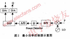
The gradient method is another method of adaptability. The signal cancellation circuit and the error cancellation circuit can use a complex baseband correlator or a bandpass correlator. The simplest iterative method is the steepest descent algorithm. In the environment of the quadratic error surface, you can choose an initial value α (defined at some points on the error surface), and then calculate the gradient of the error surface at that point, and correspondingly α Was corrected. The quadratic error surface is a classic estimation theory. The correlation between the base vr (t) and the estimated error ve (t) is equal to the gradient of the error surface. This correlation is used to drive the adaptive algorithm. The stochastic gradient signal (ve (t) vm (t) *) processed by the steepest descent method indicates that the above algorithm is adjusting α and β. When vr (t) and ve (t) are not related, the gradient is 0, which indicates that the error signal contains only distortion. The gradient method converges faster than the minimum power method and does not require constant adjustment to determine the direction of change. However, the output of the mixer is sensitive to DC offset. Like the minimum power method, the convergence time in the error cancellation circuit is longer for the same reason, which can be alleviated by compressing the linear part of the output signal before correlation.
4 Simulation process and results
In this paper, the gradient method is used to implement an adaptive feedforward linearizer. This method mainly calculates the gradient of the surface that reaches the minimum point, and uses a complex correlator to calculate the gradient. The feedforward linearizer has two loops: a signal cancellation circuit and an error cancellation circuit. The purpose of the linear cancellation circuit is to eliminate the linear part of the output signal of the power amplifier, leaving only distortion. The complex coefficient α drives a complex gain adjuster in the form of rectangular coordinates. The complex correlator is used to optimize the phase of the complex coefficients and attenuate the upper and lower branches with opposite phases. Enter the second loop. The distorted signal of the lower branch and the output of the upper branch of the power amplifier constitute an error cancellation circuit. The coefficient β adjusts the complex gain adjuster of the downstream branch so as to be opposite to the distortion phase of the upstream branch. Adopt two-way modulation signal input, the interval is 100 MHz, the carrier frequency is 1.0 GHz, α is -0.1, β is -0.01, and the iterative least mean square is used for optimization, and the rectangular coordinate vector modulator is used. For simplicity, ideal passive components are used. Choose the appropriate parameters carefully. The best way is to ensure that the signal cancellation circuit loop (α adaptation coefficient) converges to a smaller range before the error cancellation circuit loop (β adaptation coefficient) begins to converge.
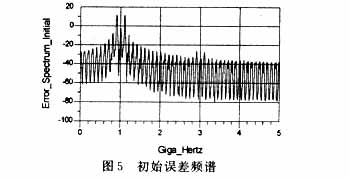
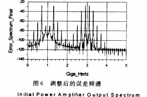
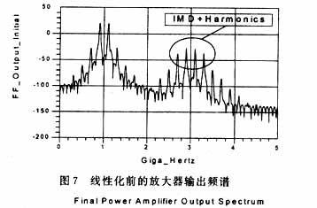
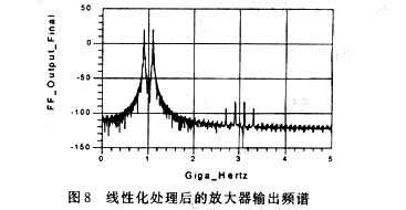
Using ADS2003 for system-level simulation, the simulation results are shown in Figure 3 to Figure 8 when the power backs up by 5 dB. Figure 3 shows the changes in the real and imaginary parts of α, β in the adaptive adjustment process. It can be seen from the figure that the adjustment process of α must precede the adjustment of β. The overall change trend of the third-order and fifth-order intermodulation can be seen from Figure 4, and it can be seen from the figure that when the adjustment continues, the third-order intermodulation improves by 40 dBc, while the fifth-order intermodulation stabilizes by 65 dBc. FIG. 5 shows the initial error spectrum, and FIG. 6 shows the adjusted error spectrum. Figure 7 shows that a large intermodulation power and harmonics are generated when the power is backed up by 5 dB. Figure 8 shows the output of the feedforward linearizer after adaptive processing. The simulation results show that after adaptive feedforward processing, the third-order and fifth-order intermodulation have been significantly improved, and the linearity of the power amplifier has been significantly improved. 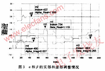

5 Conclusion
The linearization technology of RF power amplifier can obviously improve the linearity of the amplifier, and at the same time increase the output power and efficiency. Among the three linearization techniques of negative feedback, predistortion, and feedforward, feedforward technology provides the advantages of feedback, but does not have the disadvantages of instability and bandwidth limitation. In this paper, the gradient method is used to implement an adaptive feedforward linearizer. Simulation results show that the power amplifier's third-order intermodulation can improve 40dBc, and the fifth-order intermodulation can improve 65dBc when the power feedback is 5dB, compared with no adaptive feedforward adjustment. The linearity of the power amplifier is significantly improved. Achieving high-power, high-linear output, he reduced the requirements for the final stage of the power amplifier and improved the electrical efficiency of the power amplifier. In a multi-carrier, high-speed, large-capacity communication system, the feedforward amplifier can solve the adjacent channel interference, improve the system ACPR value, and ensure the effectiveness and reliability of the system.